7 reasons why you should get cozy with INDEX()

Today lets get cozy. Lets start a fling (a very long one). Lets do something that will make you smart, happy and relaxed.

Don’t get any naughty ideas. I am talking about INDEX() formula.

INDEX?!?

Of all the hundreds of formulas & thousands of features in Excel, INDEX() would rank somewhere in the top 5 for me. It is a versatile, powerful, simple & smart formula. Although it looks plain, it can make huge changes to the way you analyze data, calculate numbers and present them. It is so important that, whenever I teach (live or online), I usually dedicate 25% of teaching time to INDEX().

Enough build up. Lets get cozy with INDEX.

Understanding INDEX formula

In simple terms, INDEX formula gives us value or the reference to a value from within a table or range.

While this may sound trivial, once you realize what INDEX can do, you would be madly in love with it.

Few sample uses of INDEX

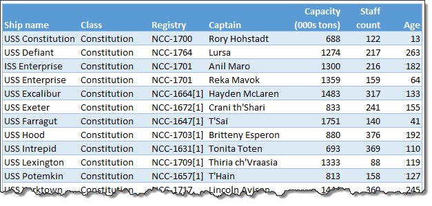
1. Lets say you are the star fleet commander of planet zorg. And you are looking at a list of your fleet in Excel (even in other planets they use Excel to manage data). And you want to get the name of 8th item in the list.

INDEX to rescue. Write =INDEX(list, 8)

2. Now, you want to know the captain of this 8th ship, which is in 3rd column. You guessed right, again we can use INDEX,

=INDEX(list, 8,3)

Syntax of INDEX formula

INDEX has 2 syntaxes.

1. INDEX(range or table, row number, column number)

This will give you the value or reference from given range at given row & column numbers.

2. INDEX(range, row number, column number, area number)

This will give you the value or reference from specified area at given row & column numbers.

It may be difficult to understand how these work from the syntax definition. Read on and everything will be clear.

7 reasons why INDEX is an awesome companion

Whether you are in planet zorg managing dozens of star fleet or you are in planet earth managing a list of vendors, chances are you are wrestling everyday with data, pleasing a handful of managers (and clients), delivering like a rock star all while having fun. That is why you should partner with INDEX. It can make you look smart, resourceful and fast, without compromising your existing relationship with another human being.

Data used in these examples

For all these examples (except #6), we will use below data. It is in the table named sf.

Reason 1: Get nth item from a list

You already saw this in action. INDEX formula is great for getting nth item from a list of values. You simply write =INDEX(list, n)

Reason 2: Get the value at intersection of given row & column

Again, you saw this example. INDEX formula can take a table (or range) and give you the value at nth row, mth column. Like this =INDEX(table, n, m)

Reason 3: Get entire row or column from a table

For some reason you want to have the entire or column from a table. A good example is you are analyzing star fleet ages and you want to calculate average age of all ships.

You can write =AVERAGE(age column)

or you can also use INDEX to generate the age column for you. Assuming the fleet table is named sf and age is incolumn 7

write =AVERAGE(INDEX(sf, ,7))

Notice empty value for ROW number. When you pass empty or 0 value to either row or column, INDEX will return entire row or column.

Likewise, if you want an entire row, you can pass either empty or 0 value for column parameter.

Reason 4: Use it to lookup left

By now you know that VLOOKUP() cannot fetch values from columns to left. It does not matter if the person looking up is the star fleet commander.

But INDEX along with MATCH can fix this problem.

Lets say you want to know which ship has maximum capacity.

1. First you find what is the maximum capacity =MAX(sf[Capacity (000s tons)])
2. Then you find position of of this capacity in all values =MATCH(max_capacity, sf[Capacity (000s tons)],0)
3. Now, extract the corresponding ship name =INDEX(sf[Ship Name], max_capacity_position)

Or in one line, the formula becomes

=INDEX(sf[Ship Name], MATCH( MAX(sf[Capacity (000s tons)]), sf[Capacity (000s tons)], 0))

For more tips read using INDEX + MATCH combination

Reason 5: Create dynamic ranges

So far, your reaction to INDEX’s prowess might be ‘meh!’. And that is understandable. You are of course star fleet commander and it is difficult to please you. But don’t break-up with INDEX yet.

You see, the true power of INDEX lies in its nature. While you may think INDEX is returning a value, the reality is, INDEX returns a reference to the cell containing value.

So this means, a formula like =INDEX(list, 8) looks like it is giving 8th value in list.

But it is really giving a reference to 8th cell.

Since the result of INDEX is a reference, we can use INDEX in any place where we need to have a reference.

Sounds confusing?

For example, to sum up a list of values in range A1:A10, we write =SUM(A1:A10)

Now, in that formula, both A1 and A10 are references.

Since INDEX gives a reference, we can replace either (or both) A1 & A10 with INDEX formula and it still works.

so =SUM(A1 : INDEX(A1:A50,10))

will give the same result as =SUM(A1:A10)

Although the INDEX route appears overly complicated, it has other applications.

Example 1: SUM of staff in first x ships

Lets say you want to sum up staff in first ‘x’ ships in the sf table.

Since ‘x’ changes from time to time, you want a dynamic range that starts from first ship and goes up to xth ship.

Assuming ‘x’ value is in cell M1 and first ship’s staff is in cell G3,

=SUM(G3:INDEX(sf[Staff count], M1))

will give the desired result.

Example 2: A named range that refers to all ship names in column A

Many times you do not know how much data you have. Even star fleet commanders are left in dark. Lets say you are building a new ship tracking spreadsheet. Since your fleet is ever growing, you do not want to constantly update all formulas to refer to correct ranges.

For example, the ship names are in column A, from A1 to An. And you want to create a named range that points to all ships so that you can use this name elsewhere.

If you define the lstShips =A1:A10, then after you add 11th ship, you must edit this name. And you hate repetitive work.

One solution is to use OFFSET formula to define the dynamic range,

like =OFFSET(A1, 0,0, COUNTA(A:A),1)

While this works ok, since OFFSET is volatile function, it will recalculate every time something changes in your workbook. Even when someone replaces a bolt on landing gear of USS Enterprise.

This will eventually make your workbook slow.

That is where INDEX comes.

You see, INDEX is a non-volatile function*.

So you can create lstShips that points to,

=A1: INDEX(A:A, COUNTA(A:A))

*Even though INDEX is non-volatile, since we are using it in defining a range reference, Excel recalculates the lstShips every time you open the file. (reference).

Reason 6: Get any 1 range from a list of ranges

INDEX has another powerful use. You can get any one range from many ranges using INDEX.

Since you are a successful, smart & resourceful star fleet commander, you got promoted. Now you manage fleet of several planets.

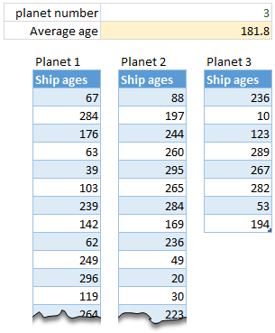
And you have similar ship detail tables for each planet in a workbook. And you want to calculate average age of any planet’s ships with just one formula.

Again INDEX to rescue.

Assuming you have 3 different tables – planet1, planet2, planet3

and selected planet number is in cell C1,

write =AVERAGE(INDEX((planet1,planet2,planet3),,,C1))

The reference (planet1,planet2,planet3) will point to all data and C1 will tell INDEX which planet’s data to use.

Pretty nifty eh?!?

Reason 7: INDEX can process arrays

INDEX can naturally process arrays of data (without entering CTRL+Shift+Enter).

For example you want to find out how much staff is in the ships whose captain’s name starts with “R”.

write =SUM(INDEX((LEFT(sf[Captain],1)=“r”)*(sf[Staff count]),0))

Although LEFT(sf[Captain],1)=”r” and sf[Staff count] produce arrays, since INDEX can process arrays automatically, the result comes without CTRL+Shift+Enter

Where as if you use SUM alone =SUM((LEFT(sf[Captain],1)=”r”)*(sf[Staff count])) you have to press CTRL+Shift+Enterto get correct results.

Other formulas: SUMPRODUCT & MATCH too can process arrays automatically.